How the Recursive Formula for Geometric Sequence Reshapes Math and Real-World Applications

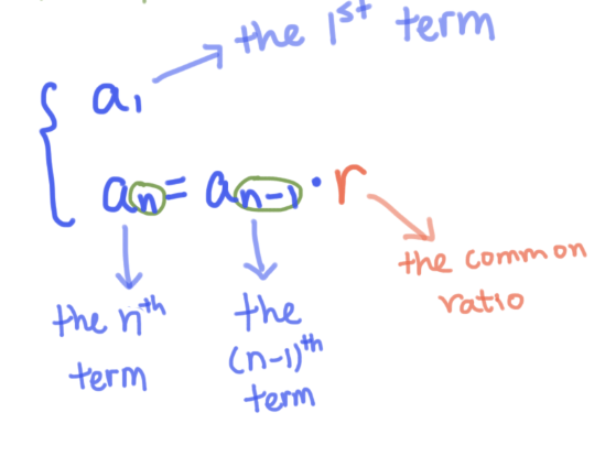
Geometric sequences are the silent architects of exponential growth, lurking in everything from compound interest calculations to the spread of viruses. Yet, while most textbooks introduce them through explicit formulas—where each term is defined as aₙ = a₁·rⁿ⁻¹—the recursive formula for geometric sequences offers a more dynamic, self-referential approach. Here, the value of a term depends not on its position in the sequence but on the one immediately before it: aₙ = aₙ₋₁·r. This subtle shift transforms how we model patterns, solve problems, and even think about recursion itself.
The power of this method lies in its adaptability. Unlike explicit formulas, which require knowing the starting term and common ratio upfront, the recursive formula for geometric sequences thrives in scenarios where only partial information is available—such as forecasting population growth with incomplete data or simulating cascading effects in network theory. It’s the mathematical equivalent of building a house brick by brick, where each new term is constructed from the last, rather than relying on a preordained blueprint.
What makes this approach particularly intriguing is its dual nature: it’s both a tool for computation and a lens for understanding iterative processes. From the Fibonacci sequence’s recursive definition to the way algorithms propagate through computer systems, the recursive formula for geometric sequences reveals deeper connections between discrete mathematics and real-world phenomena. Whether you’re optimizing a financial model or debugging a recursive algorithm, grasping this concept unlocks a precision that explicit formulas alone cannot provide.
The Complete Overview of the Recursive Formula for Geometric Sequence
At its core, the recursive formula for geometric sequences is a mathematical relationship that defines each term in the sequence based on its predecessor. For a geometric sequence with a first term a₁ and common ratio r, the recursive definition is succinct:aₙ = r·aₙ₋₁, for n > 1.
This formula encapsulates the essence of geometric progression: every term is obtained by multiplying the previous term by a constant factor r. The elegance of this approach lies in its minimalism—no need to compute all preceding terms to find aₙ; instead, you need only the immediately preceding value and the ratio.
The recursive formula for geometric sequences is not merely an alternative to the explicit form (aₙ = a₁·rⁿ⁻¹); it’s a paradigm shift. While explicit formulas are ideal for direct computation, recursive definitions excel in scenarios requiring iterative updates, such as simulations or dynamic systems. For instance, in computational finance, recursive geometric sequences model how investments compound over time without recalculating the entire series from scratch. Similarly, in physics, recursive relationships describe phenomena like radioactive decay or harmonic oscillations, where each state depends on the prior one.
Historical Background and Evolution
The concept of geometric sequences traces back to ancient civilizations, where mathematicians like Euclid and Al-Khwarizmi studied proportional relationships. However, the recursive formulation—where a term’s value is derived from its predecessor—gained prominence in the 17th century with the rise of calculus and iterative methods. Isaac Newton and Gottfried Wilhelm Leibniz, while focused on differential equations, inadvertently laid groundwork for recursive thinking by framing problems in terms of infinitesimal changes.The 19th century saw a formalization of recursive definitions, particularly in the works of Augustus De Morgan and George Boole, who explored sequences and series as tools for logical and algebraic manipulation. By the 20th century, recursive geometric sequences became a cornerstone of computer science, thanks to pioneers like Alan Turing and John von Neumann. Their work demonstrated how recursive algorithms—mirroring the recursive formula for geometric sequences—could solve complex problems efficiently, paving the way for modern programming paradigms.
Core Mechanisms: How It Works
The recursive formula for geometric sequences operates on a feedback loop: each term is a function of the one before it. For example, consider a sequence where a₁ = 3 and r = 2. The first few terms would be:Table of Contents
- The Complete Overview of the Recursive Formula for Geometric Sequence
- Historical Background and Evolution
- Core Mechanisms: How It Works
- Key Benefits and Crucial Impact
- Major Advantages
- Comparative Analysis
- Future Trends and Innovations
- Conclusion
- Comprehensive FAQs
- Q: Can the recursive formula for geometric sequences handle non-constant ratios?
- Q: How does recursion depth affect performance in geometric sequence calculations?
- Q: Are there real-world examples where the recursive formula is preferred over the explicit one?
- Q: Can negative ratios in the recursive formula lead to divergent sequences?
- Q: How is the recursive formula for geometric sequences used in algorithm design?
- Q: What are the limitations of using recursion for geometric sequences in programming?
- Q: Can the recursive formula be extended to multidimensional sequences?
This iterative process highlights the self-similarity inherent in geometric sequences—a property that recursive definitions exploit. Unlike explicit formulas, which require O(n) operations to compute the n-th term, recursive methods can leverage memoization or dynamic programming to optimize performance, especially in large-scale applications.
Moreover, the recursive formula for geometric sequences is not limited to positive ratios. When r is negative, the sequence oscillates (e.g., aₙ = (-1)ⁿ·a₁), and when 0 < r < 1, it converges—a behavior critical in modeling damping systems or probabilistic processes. This versatility makes the recursive approach indispensable in fields where sequences evolve dynamically, such as machine learning or epidemiological modeling.
Key Benefits and Crucial Impact
The recursive formula for geometric sequences is more than a mathematical curiosity; it’s a problem-solving framework. Its strength lies in its ability to model systems where change is proportional to the current state, a pattern observed in nature, economics, and technology. For instance, in algorithm design, recursive geometric sequences help optimize divide-and-conquer strategies, reducing time complexity in tasks like binary search or fast Fourier transforms.Beyond computation, this formula fosters a deeper understanding of iterative processes. It teaches us to think in terms of relationships rather than absolute values—a mindset that extends to fields like biology (population dynamics), engineering (signal processing), and even art (fractal generation). The recursive approach also aligns with human cognition, as it mirrors how we often make decisions based on past outcomes rather than fixed rules.
"Recursion is the most natural way to think about computation. The fact that it’s also the most mathematically elegant is no coincidence." — Donald Knuth, The Art of Computer Programming
Major Advantages
- Dynamic Adaptability: The recursive formula for geometric sequences adjusts seamlessly to changing ratios, making it ideal for real-time systems where parameters evolve (e.g., adaptive learning rates in AI).
- Memory Efficiency: Unlike explicit formulas, recursive methods often require storing only the last computed term, reducing memory overhead in large-scale computations.
- Algorithmic Elegance: Recursive definitions simplify complex problems by breaking them into smaller, self-similar subproblems—a principle central to algorithms like quicksort or merge sort.
- Modeling Nonlinear Growth: The formula naturally captures exponential and oscillatory behaviors, critical in fields like physics (wave functions) and finance (option pricing).
- Interdisciplinary Applications: From predicting viral spread to designing fractal antennas, the recursive geometric sequence is a unifying concept across disciplines.

Comparative Analysis
| Recursive Formula for Geometric Sequence | Explicit Formula (aₙ = a₁·rⁿ⁻¹) |
|---|---|
| Defines terms based on predecessors (aₙ = r·aₙ₋₁). | Defines terms based on position and initial conditions. |
| Excels in iterative or dynamic systems (e.g., simulations). | Ideal for direct computation when all parameters are known. |
| Requires base case (a₁) and ratio (r). | Requires a₁, r, and term index (n). |
| Prone to stack overflow in deep recursion (mitigated via tail recursion or loops). | No risk of overflow; computes any term in constant time. |
Future Trends and Innovations
As computational power grows, the recursive formula for geometric sequences is poised to play a larger role in adaptive systems. In machine learning, recursive geometric models could improve time-series forecasting by dynamically adjusting ratios based on new data. Meanwhile, quantum computing may leverage recursive sequences to optimize parallel processing tasks, where iterative updates are inherently more efficient than explicit calculations.Another frontier is bioinformatics, where recursive geometric patterns appear in DNA sequencing and protein folding. By treating genetic data as recursive sequences, researchers might uncover hidden regulatory mechanisms. Similarly, in robotics, recursive geometric algorithms could enable swarm intelligence, where each agent’s behavior is a function of its neighbors’ states—a direct application of the recursive principle.
Conclusion
The recursive formula for geometric sequences is a testament to the beauty of mathematical abstraction. It bridges theory and practice, offering a lens to view the world in terms of iterative relationships. Whether you’re a mathematician proving theorems or an engineer designing algorithms, this tool provides a framework for thinking about growth, decay, and transformation in ways that explicit formulas cannot.Its enduring relevance stems from its simplicity and versatility. As fields like AI, quantum computing, and systems biology continue to evolve, the recursive geometric sequence will remain a fundamental concept—one that connects the dots between abstract theory and tangible innovation.
Comprehensive FAQs
Q: Can the recursive formula for geometric sequences handle non-constant ratios?
The standard recursive formula (aₙ = r·aₙ₋₁) assumes a constant ratio r. For non-constant ratios, the sequence becomes a generalized geometric sequence, where the recursive relation might involve multiple terms (e.g., aₙ = rₙ·aₙ₋₁). Such cases are common in stochastic processes or adaptive algorithms.
Q: How does recursion depth affect performance in geometric sequence calculations?
Deep recursion can lead to stack overflow errors, as each recursive call consumes memory. To mitigate this, use tail recursion (where the recursive call is the last operation) or convert the recursion to an iterative loop (e.g., while loop). Many programming languages optimize tail recursion, but explicit loops are generally safer for large n.
Q: Are there real-world examples where the recursive formula is preferred over the explicit one?
Yes. In financial modeling, recursive geometric sequences simulate compound interest without recalculating the entire series. In computer graphics, recursive subdivision (e.g., fractals) generates complex shapes by repeatedly applying a geometric ratio. Even in epidemiology, recursive models predict disease spread based on current infections.
Q: Can negative ratios in the recursive formula lead to divergent sequences?
Negative ratios (r < 0) produce oscillating sequences (e.g., 3, -6, 12, -24,...), but they remain bounded if |r| < 1. For |r| ≥ 1, the terms grow in magnitude, potentially diverging. However, the sequence is still well-defined recursively—divergence is a property of the explicit form’s behavior as n → ∞.
Q: How is the recursive formula for geometric sequences used in algorithm design?
Recursive geometric sequences underpin algorithms like the exponential search (used in binary search variants) and fast multiplication (e.g., Karatsuba algorithm). They also appear in dynamic programming problems where subproblems share overlapping substructure, such as the Fibonacci sequence or shortest-path calculations.
Q: What are the limitations of using recursion for geometric sequences in programming?
Limitations include:
- Stack Overflow: Deep recursion exhausts memory.
- Performance Overhead: Recursive calls introduce function call overhead.
- Debugging Complexity: Recursive logic can be harder to trace than iterative loops.
Q: Can the recursive formula be extended to multidimensional sequences?
Yes. In multivariate geometric sequences, each term depends on multiple predecessors, often defined via matrices or tensors. For example, a 2D geometric sequence might satisfy aₙ = r₁·aₙ₋₁ + r₂·bₙ₋₁, where bₙ is another sequence. This extends to vector recursion in linear algebra and tensor networks in quantum computing.
Leave a Comment
Comments are moderated before appearing. The data you submit is processed according to the Privacy Policy of Sac.