The Hidden Power of How to Compute Interquartile Range in Data Mastery
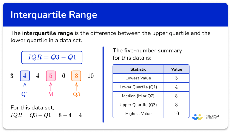
Data doesn’t lie—but it can mislead if misinterpreted. The interquartile range (IQR) stands as a silent guardian against skewed conclusions, offering a sharper lens than the mean or standard deviation. While many analysts default to averages, the IQR reveals the true spread of the middle 50% of data, stripping away the noise of extreme values. This is why understanding how to compute interquartile range isn’t just a technical skill; it’s a strategic advantage in fields from finance to healthcare.
The problem? Most tutorials treat the IQR as a mechanical formula—plug in numbers, get an answer. But the real insight lies in its purpose: to measure dispersion without distortion. Whether you’re identifying outliers in clinical trials or assessing market volatility, the IQR’s robustness makes it indispensable. Yet, its calculation isn’t universally understood. Even seasoned professionals often stumble over the nuances of quartile definitions or the impact of dataset size. This gap isn’t just academic; it translates to flawed risk assessments, misallocated resources, or overlooked anomalies.
Consider this: A dataset’s median might appear stable, but its IQR could signal hidden instability. A stock portfolio’s returns may average 8%, yet the IQR might expose a 20% swing between the 25th and 75th percentiles—information critical for investors. The key to leveraging this tool lies in mastering how to compute interquartile range with precision, recognizing when to apply it, and interpreting its implications beyond the raw number.
The Complete Overview of How to Compute Interquartile Range
The interquartile range (IQR) is a measure of statistical dispersion, representing the range within which the central 50% of data points lie. Unlike the total range (max–min), which is sensitive to outliers, the IQR focuses on the interquartile spread—Q3 minus Q1—where Q1 is the first quartile (25th percentile) and Q3 is the third quartile (75th percentile). This method is foundational in box plots, outlier detection, and robust statistical analysis. Its strength lies in its resistance to skewness, making it a preferred metric in fields where extreme values can distort interpretations.
To compute interquartile range, one must first determine the quartiles. However, the process isn’t uniform: different statistical traditions (e.g., Tukey’s hinges, linear interpolation) yield slightly varied results. For example, in a dataset of 10 values, Q1 might be the average of the 3rd and 4th values, while in a dataset of 11, it’s the 3rd value itself. This variability underscores the importance of consistency in methodology, especially when comparing datasets or industries. The IQR’s calculation, therefore, isn’t just about arithmetic—it’s about contextual rigor.
Historical Background and Evolution
The concept of quartiles emerged in the 19th century as statisticians sought to quantify data distribution beyond simple averages. Early work by Francis Galton and Karl Pearson laid the groundwork for percentiles, but it was John Tukey who, in the mid-20th century, formalized the IQR as a tool for exploratory data analysis (EDA). Tukey’s approach—using the median of halves to define quartiles—became a cornerstone of robust statistics, particularly in fields where outliers were prevalent, such as engineering and economics.
Table of Contents
- The Complete Overview of How to Compute Interquartile Range
- Historical Background and Evolution
- Core Mechanisms: How It Works
- Key Benefits and Crucial Impact
- Major Advantages
- Comparative Analysis
- Future Trends and Innovations
- Conclusion
- Comprehensive FAQs
- Q: Why is the interquartile range more reliable than the standard deviation for skewed data?
- Q: Can the IQR be used to identify outliers?
- Q: How does sample size affect the calculation of quartiles?
- Q: Is the IQR affected by the order of data points?
- Q: What industries benefit most from using the IQR?
Over time, the IQR’s utility expanded beyond academia. In the 1980s, its adoption in quality control (e.g., Six Sigma) demonstrated its practical value in manufacturing, where process variability directly impacted product consistency. Today, the IQR is a standard in software like R and Python (via libraries like NumPy and Pandas), embedded in algorithms for anomaly detection and even machine learning preprocessing. Its evolution reflects a broader shift toward statistical methods that prioritize resilience over sensitivity.
Core Mechanisms: How It Works
The calculation of the IQR hinges on two steps: identifying the quartiles and computing their difference. For Q1 (the first quartile), you locate the 25th percentile of the dataset, while Q3 marks the 75th percentile. The IQR is then Q3 − Q1. However, the method for interpolating quartiles varies. For instance, the "nearest rank" method assigns Q1 to the value at position 0.25 × (n + 1), where n is the dataset size, while the "linear interpolation" method averages adjacent values if the position isn’t an integer.
Consider a dataset of exam scores: [60, 70, 75, 80, 85, 90, 95, 100]. To compute interquartile range, Q1 is the median of the lower half ([60, 70, 75, 80]), which is (70 + 75)/2 = 72.5, and Q3 is the median of the upper half ([85, 90, 95, 100]), which is (90 + 95)/2 = 92.5. The IQR is 92.5 − 72.5 = 20. This approach ensures that the middle 50% of scores are captured, providing a clearer picture of central tendency than the full range (100 − 60 = 40).
Key Benefits and Crucial Impact
The IQR’s primary advantage is its resistance to outliers. While the mean can be dragged by extreme values, the IQR remains anchored to the dataset’s core distribution. This makes it invaluable in fields like finance, where a single volatile trade might skew average returns, or in healthcare, where a few extreme patient responses could distort treatment efficacy metrics. By focusing on the interquartile spread, analysts gain a more reliable measure of variability, reducing the risk of misleading conclusions.
Beyond robustness, the IQR is a gateway to deeper insights. It’s the backbone of box plots, which visually separate data into quartiles, medians, and outliers. In quality assurance, an IQR of 5 in a manufacturing process might trigger investigations into consistency, whereas a standard deviation of 10 might not. Its applications extend to sports analytics (e.g., tracking athlete performance variability) and climate science (e.g., analyzing temperature ranges). The IQR isn’t just a number—it’s a diagnostic tool for understanding data’s true behavior.
"The interquartile range is the only measure of spread that doesn’t require assumptions about the underlying distribution of the data." — George Casella, Professor of Statistics
Major Advantages
- Outlier Resistance: Unlike the range or standard deviation, the IQR ignores extreme values, providing a stable measure of dispersion.
- Percentile Focus: By targeting the 25th and 75th percentiles, it highlights where the bulk of data resides, not just the extremes.
- Box Plot Integration: The IQR defines the "box" in box-and-whisker plots, offering a visual representation of data spread.
- Non-Parametric: No assumptions about data distribution (e.g., normality) are needed, making it universally applicable.
- Actionable Insights: In industries like logistics, a widening IQR might signal increasing variability in delivery times, prompting process reviews.

Comparative Analysis
| Metric | Interquartile Range (IQR) |
|---|---|
| Purpose | Measures spread of the middle 50% of data; robust to outliers. |
| Calculation | Q3 − Q1 (where Q1 = 25th percentile, Q3 = 75th percentile). |
| Sensitivity to Outliers | Low; ignores extreme values. |
| Use Cases | Outlier detection, box plots, non-normal data analysis. |
| Limitations | Does not account for full data range; less intuitive than standard deviation for some audiences. |
Future Trends and Innovations
The IQR’s role is evolving alongside big data and machine learning. As datasets grow in complexity, traditional quartile methods are being augmented by adaptive algorithms that dynamically adjust for skewed distributions. For example, in high-frequency trading, analysts now use IQR-like metrics in real-time to flag anomalies within milliseconds. Meanwhile, in healthcare, AI-driven IQR analysis is identifying patient response patterns that human statisticians might overlook.
Emerging trends also include the integration of IQR principles into automated outlier detection systems. Tools like Python’s `scipy.stats` now offer enhanced quartile calculation methods, and cloud-based analytics platforms (e.g., Google BigQuery) are embedding IQR-based diagnostics into their workflows. As data literacy becomes a corporate priority, the IQR’s clarity and precision will likely position it as a staple in data-driven decision-making, bridging the gap between statistical theory and practical application.

Conclusion
The interquartile range is more than a statistical formula—it’s a lens through which data’s true nature is revealed. By focusing on the middle 50%, it cuts through the noise of outliers and skewed distributions, offering a clearer view of variability. Whether you’re a data scientist refining predictive models or a business analyst assessing risk, understanding how to compute interquartile range equips you with a tool that’s both precise and adaptable.
Yet, its power lies not just in calculation but in interpretation. A widening IQR might signal increasing volatility; a narrow IQR could indicate consistency. The key is to move beyond rote computation and ask: What does this spread tell me about my data’s behavior? In an era where data is abundant but insights are scarce, the IQR remains a reliable compass—one that, when mastered, transforms raw numbers into actionable knowledge.
Comprehensive FAQs
Q: Why is the interquartile range more reliable than the standard deviation for skewed data?
A: The standard deviation is highly sensitive to outliers and assumes a normal distribution. The IQR, by contrast, focuses on the central 50% of data, making it robust against skewness and extreme values. For example, in a dataset with a few very high values, the standard deviation will inflate, while the IQR remains stable.
Q: Can the IQR be used to identify outliers?
A: Yes. A common rule is to flag values below Q1 − 1.5 × IQR or above Q3 + 1.5 × IQR as outliers. This method is widely used in box plots and exploratory data analysis to detect anomalies without assuming a distribution.
Q: How does sample size affect the calculation of quartiles?
A: Sample size influences whether quartiles are calculated using exact positions or interpolation. For small datasets (<20 values), methods like Tukey’s hinges (median of halves) are precise, while larger datasets often use linear interpolation. The choice of method can slightly alter the IQR, so consistency is critical when comparing datasets.
Q: Is the IQR affected by the order of data points?
A: No. The IQR is based on percentiles, which are order statistics. Sorting the data first ensures accurate quartile calculation, but the final IQR value remains unchanged regardless of the original order.
Q: What industries benefit most from using the IQR?
A: Industries with high variability or non-normal data benefit most, including finance (risk assessment), healthcare (patient response analysis), manufacturing (quality control), and sports analytics (performance tracking). The IQR’s robustness makes it ideal for scenarios where outliers are common or distribution assumptions are unreliable.
Leave a Comment
Comments are moderated before appearing. The data you submit is processed according to the Privacy Policy of Sac.